Semicircles from Sequences
Some time ago, I happened across this lovely YouTube video about the Recamán sequence. The video was made by a channel called Numberphile, and if you're not familiar with their videos, they're very worth checking out. The Recamán sequence, as described in the video, is infinite and nonmonotonic, and there is a uniuqe set of rules for generating it, but that exact entity and its rule set aren't what I'm interested in here.
What I'm really interested in is the sequence visualization method demonstrated in that video. For any sequence, you take the 0th element and the 1st element, put them on the real number line, and draw a half circle between them with its end points on each of the elements -- let's demand that this initial half circle "point" upwards, just to remove ambiguity. Then you draw a downward-pointing half circle between the 1st and 2nd elements in the sequence, an upward one between the 2nd and 3rd, etc. So every sequence element is connected to its two adjacent elements by inverted half circles. The following image shows a few toy examples of this, to really drive the point home. Note that the three sequences in the image are not necessarily drawn on the same number line as each other. Some amount of translation and scaling has taken place on each, but try and convince yourself that they were made from their respective sequences using the method just described.
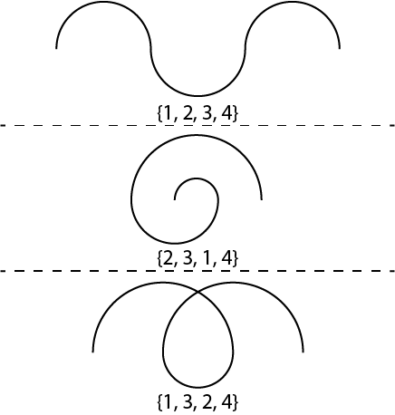
This procedure really struck me when I first saw it. You can plot some portion of a sequence and get a sense for what its behavior is, just at a glance. It's kind of like a sloppy fingerprinting technique for the sequence. So let's generate images from some familiar sequences and see how they look!
A Couple Example Sequences
The Primes
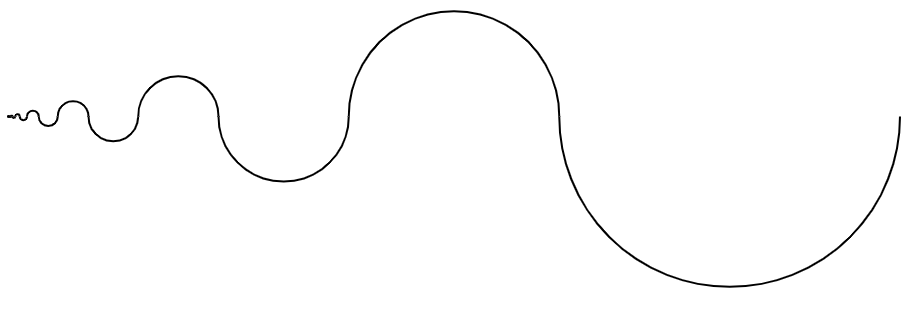
First let's take a look at some primes. I've plotted here the sequence made up by the first 50 primes.

One cool thing to note is that you can get a sense of the distribution of early twin primes at a glance. They are represented by the those really narrow hills and valleys.
The Fibonacci Sequence
How about the first twenty Fibonacci numbers.
This is probably what you would expect to see. The gap between two successive Fibonacci numbers always increases, so the drawing is dominated by the rightmost arc, and the details coming from the early numbers are lost in the image rescaling that the largest arc requires. An interesting thing to note is that (as long as automatic scaling is applied to the image), the image resulting from the first 100 or 1000 Fibonacci numbers looks identical to the one shown above. This is because the ratio of two successive Fibonacci numbers \(a_{n}/a_{n-1}\) converges to the constant \(\varphi\) for large \(n\), so the spacing will always appear the same as you add more elements, as long as you start with \(n\) sufficiently large.
The Gray Code
If you're not farmiliar with the Gray code (also called reflected binary), it's an alternate binary encoding for numbers. Specifically it's an encoding where two integers \(n\) and \(n+1\) only differ by a single bit flip. This encoding finds use in error correcting code and in removing hardware race conditions. There is a sequence that is generated by reading successive gray numbers as if they were encoded in standard \(2^n\) style binary, and I want to show it, because I think it looks very nice -- a bit like lace.
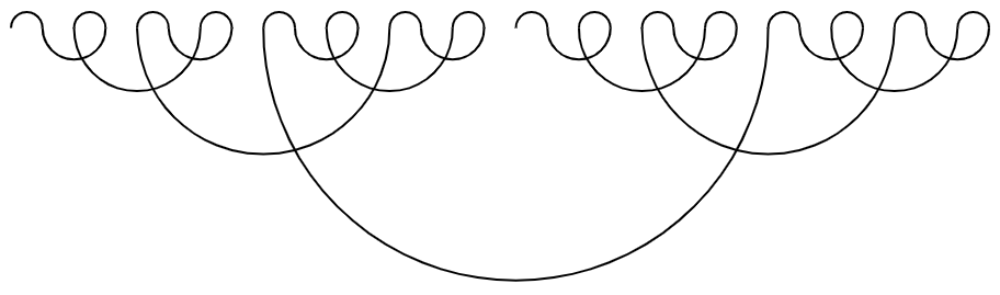
The first 32 elements are shown here. You can see that there's some self-similarity going on, as well as 2-fold symmetry at various scales, and this is maybe not too surprising, given what the sequence represents.
Imperfect Cycles
Modular Forms
A great many of the sequences studied in number theory, especially the more well known ones, increase monotonically, and \(a_n-a_{n-1}\) increases monotonically as well. That means that when you make an arc image out of them, the rightmost arc dominates the image, and it's not that interesting to look at. So what happens if we demand that the sequence doesn't really go anywhere? One of the simplest ways to do that is to generate a sequence using modular arithmetic. Let's try
\(a_n=rn\mod d\),
where \(r\) is some rational number of our choosing, and \(d\) is the denominator of the division. That is to say that \(a_n\) is the remainder of \(rn/d\). The purpose of \(r\) is to control how quickly we get through the cycle -- it's a rate parameter. Let's generate the first 10 elements of the sequence, using \(r=1.12\) and \(d=3\).
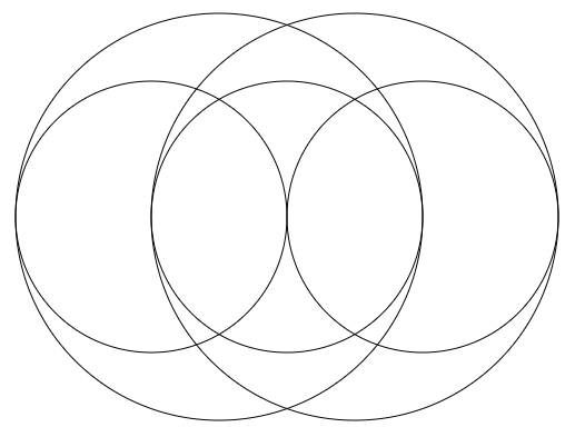
First 10 elements using r=1.12 and d=3.
Because we're taking a fractional remainder after dividing by 3, leftmost coordinate the sequence is allowed to take on is 0, and the rightmost allowed coordinate approaches but does not include 3. You can see that the arcs have two distinct sizes. The first three elements of the sequence are 0, 1.12, and 2.24, and these generate the first two arcs, which are the same size. The next element is the remainder of 3.36/3, which is just 0.36, so there is a large arc that jumps back to this from 2.24. Every time a value gets too big, it has to make the jump back, and where it's jumping back from gets shifted a bit each time.
The number of terms generated has a pretty big impact on the final look of the image. Leaving everything else alone and increasing only the number of sequence terms produces the following.
First 80 elements using r=1.12 and d=3.
This image has so many unique arcs, because the cycle is imperfect for a while. It continues trying to get to the starting point, but \(r=1.12\) prevents that from happening for quite some time. If we allow \(r\) to be an integer, we get somewhat more predictable results.
First 30 elements using r=3 and d=13. First 11 elements using r=3 and d=5.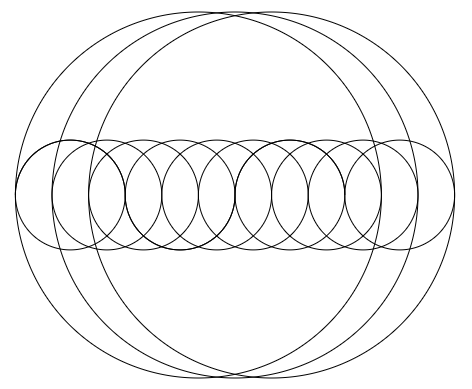
Trigonometric Functions
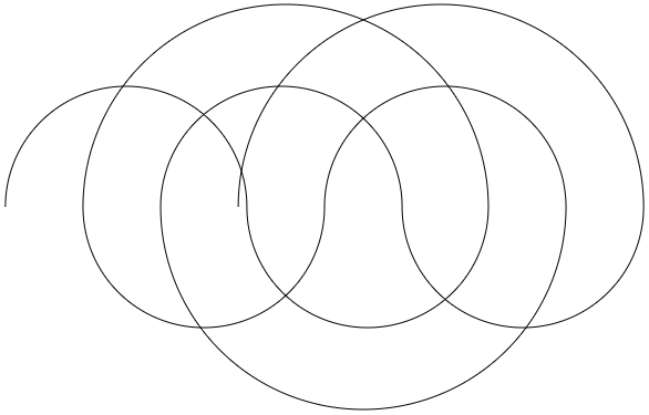
Let's try out the sequence defined by \(a_n=\cos(rn)\), where \(r\) is again arbitrarily chosen. We should expect the result to be a lot more elaborate, as cosine is in a sense doing a lot more work in its mapping than the simple division done by modulo. We should therefore expect to see arcs of more than just 2 distinct sizes.
First 150 elements using r=1.
Setting \(r\) closer to \(\pi\) has the effect of making the drawing more round and less baguette-like, and that makes sense, given what the sequence would look like if \(r=\pi\).
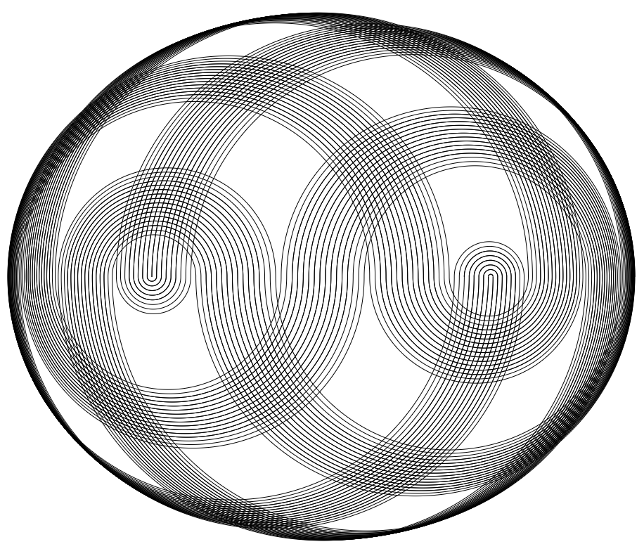
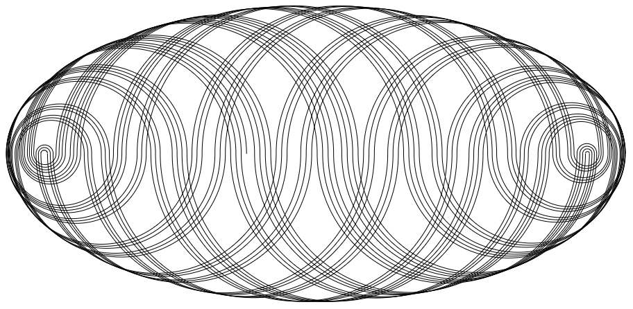
First 300 elements using r=2.
You can see in the image above that Moiré patterns are starting to show up in dense areas. Let's see if we can exaggerate that by adding more terms to the sequence.
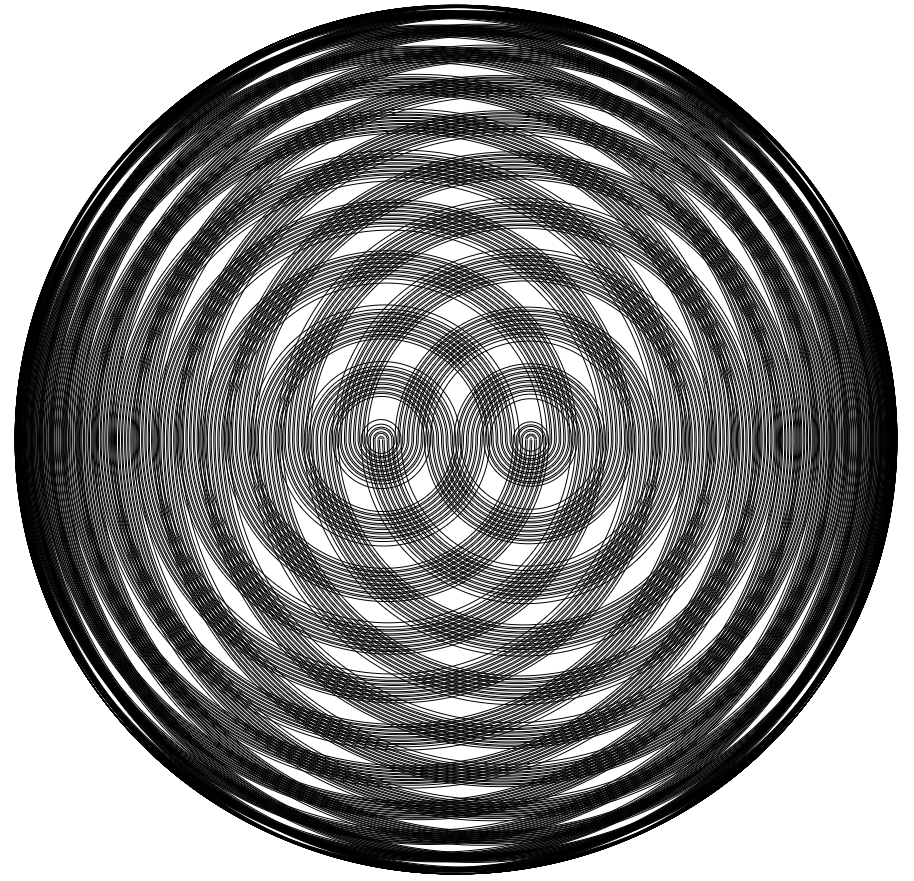
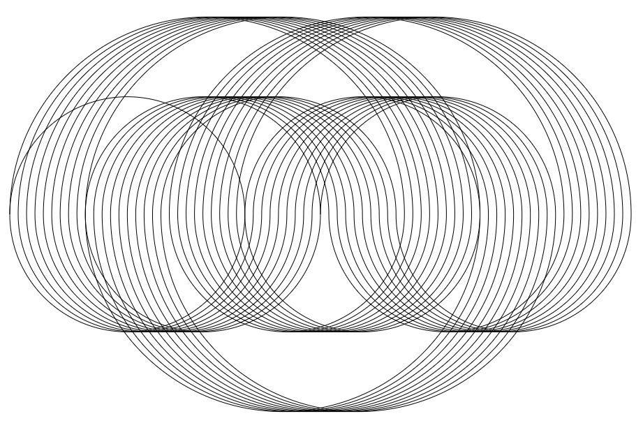
First 700 elements using r=2.8.
How Can I Play With This?
I hope I've managed to pique your curiosity and convey some of my excitement in exploring this method of sequence visualization. If you would like to generate some of these image for yourself, or try different sequence generators, periodic or not, I've put a demo on codepen, where the JavaScript is exposed. Feel free to email me if you think of a fun way to make use of this or generate something really cool.